The Bugs Were Bigger Than the Signal
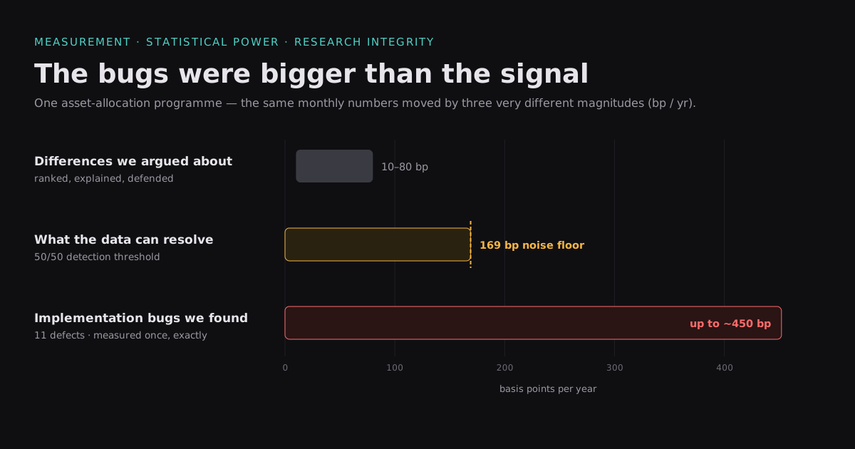
We spent weeks arguing about whether one asset-allocation model beat another by twenty basis points a year.
Then we measured what our data could actually resolve.
The answer was 169 basis points.
Every difference we had been ordering, ranking and explaining was between ten and eighty. We had been doing statistics on noise. Meanwhile the implementation defects we kept finding (and we found eleven of them) were moving the same numbers by hundreds of basis points.
The bugs were bigger than the signal. By a lot.
This is a post about what that does to a research programme, and about the one diagnostic that would have told us on day one.
First, measure the instrument
The programme had 341 monthly observations of a return difference: strategy A minus strategy B, month by month. Standard deviation 1.34% per month.
Instead of reasoning about power, we injected known effects into block-bootstrap resamples of the actual series (4,000 draws per cell) and asked how often each was distinguishable from zero.
| true effect | detected |
|---|---|
| 10 bp/yr | 6% |
| 50 bp/yr | 9% |
| 100 bp/yr | 21% |
| 169 bp/yr | 50% |
| 254 bp/yr | 80% |
The zero row came back at 4.7%, so the test was correctly sized.
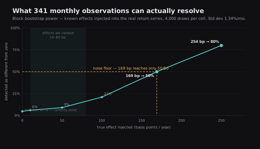
Then the sobering arithmetic. Power scales with the square root of the sample. The effect we most wanted to resolve was 73 bp/yr. Getting that to fifty-fifty would take about 1,830 months (152 years). Waiting a decade moves the threshold from 169 bp to 145 bp.
For effects that size, statistical significance is not a goal. It is not reachable.
That single table reframed everything. It relocated the work and left it valid. And it meant that the most valuable thing we had produced was not any finding about markets.
Eleven ways to be wrong
Here is the actual list, in the order we found them. Each one had already produced a number we had written down and believed.
A window that excluded the thing being tested. Our first verdict ("the optimiser is not a better teacher") came from 206 months that contained no financial crisis. The model was built for crises.
Comparing models at different risk levels. A 4.52%/yr gap shrank to 1.09% once both arms were levered to the same volatility. Three quarters of it was risk budget alone.
Comparing models under different mandates. One model was capped at 55% equity; the other spent 163 of 345 months above that. The "ceiling" we had attributed to the model was a constraint in a config file.
A proxy that correlated beautifully and was the wrong asset. Our long-Treasury series scored 0.897 correlation against the real instrument, and a volatility ratio of 0.318. It was an aggregate bond index standing in for a 20-year Treasury, on the largest position in the portfolio. Correlation cannot see a scale error.
A non-differentiable penalty under a gradient solver. The optimiser minimised
-sharpe + penalty × |w − w_prev|. That absolute value is not differentiable, and
SLSQP is a gradient method. From identical inputs, four starting points returned equity
weights of 0.132, 0.132, 0.400 and 0.221, with objective values spanning 1.2e-4 and
every one reporting success.
A unit mismatch that manufactured a result. Our covariance helper returned daily covariance. Our benchmark annualised by 252. Comparing them produced a confident "30% improvement" for every variant we tested. It was a scale error, 192× wide.
Padding a missing asset with zeros. Three assets had no history in the window, so we filled them with a constant 0.0 return to keep the matrix square. A constant column has zero variance, which a risk-minimising optimiser reads as a free risk-free asset. It bought them. Up to 45% of the portfolio, in assets that did not trade.
Constraints that absorbed the thing we were measuring. The portfolio bounds suppressed 27% of the weight dispersion between the estimators we were comparing, before any return was computed. Three separate null results had been measured through that filter.
Counting how often a constraint binds. One bound was active in 78% of months, which reads as a constraint doing constant work. We solved the unconstrained problem alongside it: the median distance between what the optimiser wanted and what the bound allowed was below 1e-5. It was resting against the bound, with the decision unchanged.
Comparing universes with different start dates. Adding two assets lifted the edge over baseline from 73 bp to 176 bp, an apparent 103 bp improvement. But the two assets start later, so the comparison also shortens the window. Running the same seven-asset model on those shorter windows accounted for 46 of the 103 bp: the later sample was simply easier. Only the remainder is attributable to the assets, and we would have reported roughly double the effect without that control.
An aggregate that hid a single year. The remaining increment was +0.39%/yr. Removing its best year took it to −0.008%, less than a basis point, in the other direction. The entire result was one gold rally, in the most recent year available, with no out-of-sample period after it.
The distinction that saved the programme
When you learn that your data cannot resolve 170 bp, the natural reaction is to conclude that nothing you measured was real.
That reaction is wrong, and the reason matters.
Look again at the eleven. They are properties of code, data and construction, distinct from effect sizes estimated from noisy returns:
- a correlation of 0.897 with a vol ratio of 0.318
- four solver answers from four starting points
- 45% of a portfolio in non-existent assets
- a 192× unit mismatch
- a median excursion below 1e-5
Those are arithmetic. You measure them once, exactly, and they are either true or not. No sample size enters.
So the honest summary is: the findings about our own machinery were solid and large; the findings about markets were small and unresolvable. Those are different categories of claim and they need different standards.
Most of what we would defend from this work falls in the first category.
Nulls arrive at the end of a chain
Here is the structure that eventually made sense of it:
evidence → representation → estimator → allocator → constraints → outcome
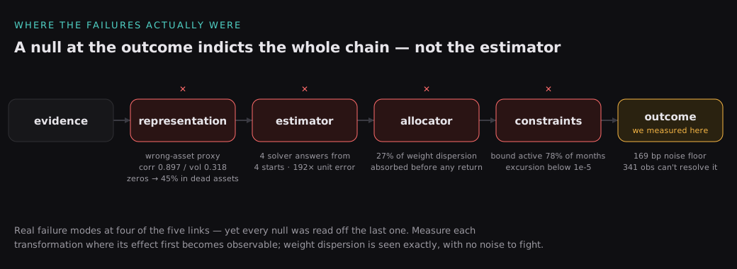
We found real failure modes at four of those five links. And critically, we kept measuring at the last one.
A null measured on portfolio returns is a statement about the whole chain, including a 27% attenuation at the allocator and a 169 bp noise floor at the outcome, and it covers more than the estimator at the start of the chain.
Once we started measuring each transformation where its effect first becomes observable, questions resolved fast. Weight dispersion is observed exactly: no standard deviation to fight. One run on weights settled a question that three return-based experiments could not.
The rule we wrote down:
Evaluate every transformation at the level where its effect first becomes observable. Do not use a noisy downstream outcome to infer that an upstream intervention had no effect.
What actually generalises
A handful of these are not about portfolios at all.
Identify a series apart from its name. Regress it against several candidate
references and check which matches at ~1.0 on both moments. A field called
bond_total_return was an aggregate index.
Report the second moment, always. Correlation is blind to scale. Two series with the same sign pattern and a 3× volatility difference correlate highly.
Regression is the wrong tool for a stand-in. A fitted value has variance R²·var(y), so least squares systematically shrinks volatility. If you need a proxy to behave like the thing, match its moments; minimising its tracking error is the other objective. Those are different objectives and the lower-tracking answer is the worse proxy.
Identical output across a swept parameter is a dead parameter. We once produced 28 byte-identical configurations and nearly concluded the parameter didn't matter. A monkeypatch couldn't reach its target, and a bound clamped instead of replacing.
Attribute the contrast between the arms. Both arms in our last experiment survived best-year removal comfortably, at +0.29% to +1.19%. The difference between them, which was the actual claim, collapsed to nothing.
A constraint touching the optimum didn't necessarily change the decision. Measure the counterfactual excursion beyond the bound; the frequency of touching it is secondary.
Freezing a result without closing it
We ended with a ledger: every claim, its status, its concentration, its boundary sensitivity, how it moved across data representations, and (this is the part we'd recommend) a revisit trigger.
Statuses came out at 12 supported, 5 suggestive, 11 not demonstrated, 13 withdrawn.
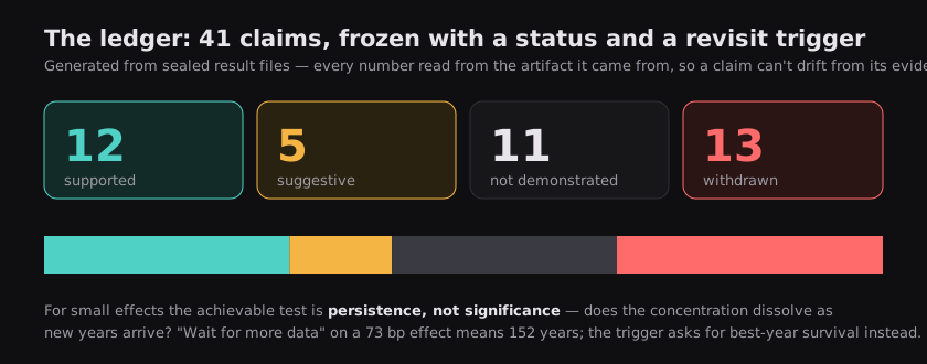
The triggers matter because "wait for more data" is usually a lie. For a 73 bp effect it means 152 years. So the triggers say what would actually change the answer, leaving wait for significance unsaid:
the increment is 100% one year: rerun when three or more further years exist, and ask whether it survives best-year removal, with clearing a t-statistic set aside.
For small effects the achievable test is persistence. Does the concentration dissolve as new years arrive, or does it stay concentrated?
The ledger is generated from sealed result files, with the status judgements in code and every number read from the artifact it came from. A claim cannot drift away from its evidence, and a stale number shows up as a missing key, visible as a gap in the artifact.
The uncomfortable part
One decision in this programme looks much better in hindsight than it felt at the time.
We refused to fabricate long histories for two assets we didn't have data for. We recorded them as unavailable and moved on, which felt like giving up evidence.
When the real instruments finally entered the analysis, they revealed no missing historical advantage at all. Their apparent value was one rally in the most recent year.
Saying "we don't have the evidence" cost us almost nothing. Manufacturing it would have produced a confident, wrong answer about the mechanism we were studying, and we would have had no way to find out.
That is the whole post, really. Most of what looked like signal was either a bug or below the noise floor. The way we found that out was by measuring our instruments as carefully as we measured the market, and by being willing to say not demonstrated about a number we liked.